Gaussian integration

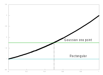
Gaussian integration is explained in several textbooks on numerical methods (Lanczos, 1957; Scheid, 1968). The basic idea is to compute the rate at positions in the total integration interval area as representative as possible. In its simplest form, the Gaussian one-point method, one single value of the rate is taken halfway through the integration interval. It gives a more accurate result than the rectangular integration method, because errors left and right of the evaluation point in the center practically cancel.

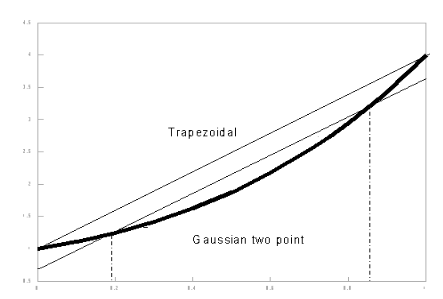
In a more formal analysis the integration interval is normalized to unity, and centralized between x=-½ and x=½. The polynomial given by y=a+bx+cx2+dx3 ... will have value a at the center point x=0. Therefore, the integrated value obtained by the one point Gaussian integration, will also be equal to a. Analytical integration of the polynomial term by term shows that the integrals of all odd terms disappear around x=0, That means that the one-point method not only exactly integrates y=a, but also y=a+bx. Similarly the two-point method will exactly integrate y=a+bx+cx2 and y=a+bx+cx2+dx3. The next step is the three point method which will enable exact integration of the fourth order term (and automatically the fifth as well).

 Rectangular - Gaussian one point - integration method.                                                                                       Trapezoidal - Gaussian two point - integration method.

Gaussian three point integration method.

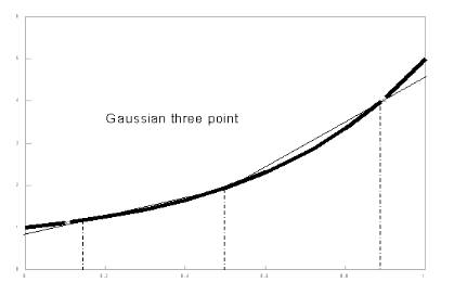
The three points of the Gaussian numerical integration are situated symmetrical around x = 0, in order to integrate the interval [-0.5,0.5]. Therefore, one of the three function evaluation points will be at the center, x=0. The other two points will be located at either side of the Y-axis at distance γ (so x=-γ and x=γ). Now the interval [-0.5 ,0.5] is divided in three parts, around these three points. The lengths of these sub-intervals determine the weights which must be imposed on the Y-values corresponding to these three x-values and considered representative for their sub-interval. Because of the symmetry again, the weights belonging to -γ and γ are equal. When these weights are considered 1, the weight of the central sub-interval is equal to ω.

The values of the relative distance γ and of the weight ω can be derived from the requirement that both the second and the fourth order terms of the polynomial will be exactly integrated (Goudriaan, 1986):

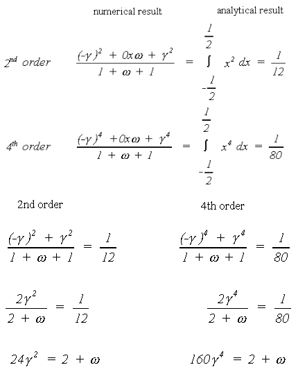
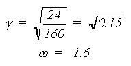
Substitution yields the following values for the relative distance and the weight:

Created with the Personal Edition of HelpNDoc: Free iPhone documentation generator